Author: Skillwave
If you’ve worked with Excel for any length of time, it’s almost certain that you’ve ended up with one table that has your base information, and a few more tables that contain related records. We call those other tables “lookup” or “reference” tables as they contain the missing information that we often want to pull into our main data table, allowing us to make better use of Excel’s rich toolsets. This process is commonly called enriching a table or de-normalizing a table, and is solved by most Excel users via a combination of formulas including:
This time, we’re going to create a dynamic process with Power Query that runs faster and is more intuitive than VLOOKUP. So prepare to say goodbye to the VLOOKUP era and say hello to Power Query for Excel
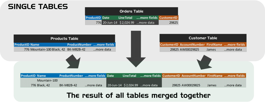 We have three single tables that we want to merge together:
Our goal is to merge all three tables using the Orders table as our base, adding the related records and attributes from the other two tables to each row from the Orders table. Our end result will be one large table with all the related columns housed together.
In our scenario, our data is already highly organized for us, with all tables defined as tables in Excel. So our next step is to take advantage of that, and create pointers to those tables inside Power Query.
In order to reference those tables in Power Query we:
For this second part all we have to do is reference our base table (or query) and in this case we’re going to use our Orders table as our base.
We go to the Power Query tab and select Show Pane so we can see the Query Pane on our right hand. Then we right click on the Orders query and select Reference.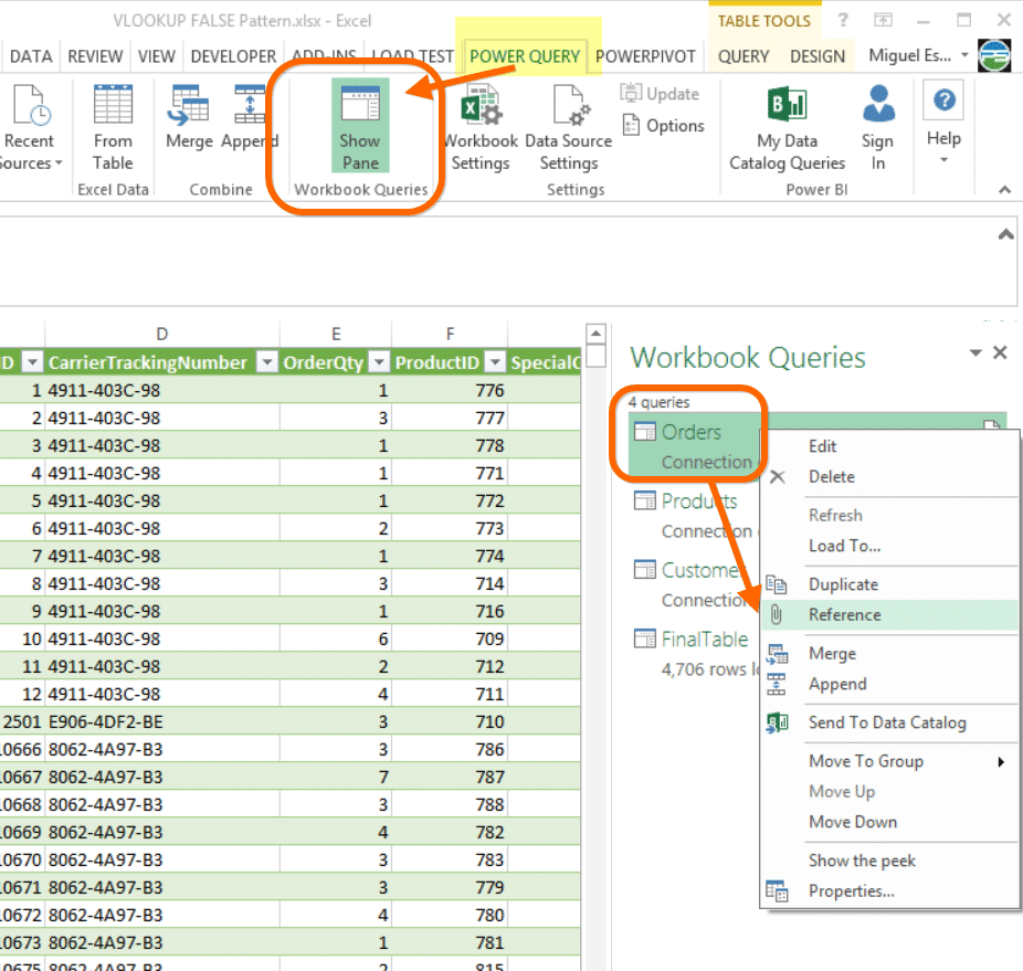
This essentially just pulls the results of the first query into a completely new query, which you’ll see in the Query Pane as Orders (2). Right click that new query and choose Edit to start the merging process.
Once you’re in the Power Query Editor Window, click the Merge button. This will pop up a new window that will guide us through the process of merging our tables together.
We need to define which table to merge with our current table and which columns contain the info to be matched.
This is the tricky part of the merge. Like working with VLOOKUP, we are trying to take a table that has a column with many values in it, and look up those values in a column that has a unique list of values. It’s important that your base query starts as the “many” side of the relationship, and that your “lookup” column is the “one” side of the relationship.
In this case our Orders table has many products in it, but our Products table has a unique list of products. So in the bottom portion of the window, we’ll choose to merge the Products table with our base table (Orders).
Next we need to identify the column that is common between the two tables (ProductID in this case). Then we simply select the ProductID columns in both tables so that they are highlighted, and click OK.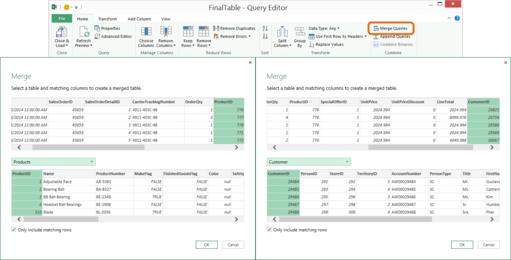
Repeat the same process to Merge the Customer table on the CustomerID column as shown in the picture above. The result should look a bit like this: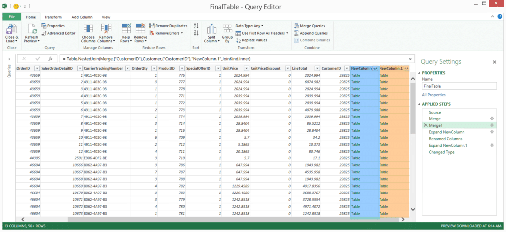
As you can see from the picture above, we added two columns containing the word Table in a green font. But it’s more than just a word… these are actually truly tables that contain each row of data from the corresponding rows of the Customer and Products Table!
We can peek inside by clicking the white space beside the word table, or we can expand those tables so we can get the columns from each.
Now that we know what’s inside of those table values for each row, let’s expand them into columns. Simply click on the directional arrows icon next to the name of the column to Expand the column, as shown in the following image:
From the picture above, you can see that you are able to choose which columns you want to keep, and which you don’t want. (Un-check the box that states Use original column name as prefix, or you’ll get columns named NewColumn.ProductID instead of just ProductID!)
Expand the other column as well – and don’t forget to un-check the Use original column name as prefix box again if it’s checked.
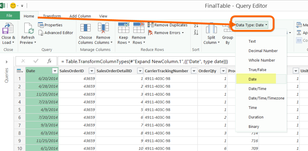
The final step of our cleanup is to force the Date column’s data type. Select the Date column, go to the Home tab, and set the data type to Date:
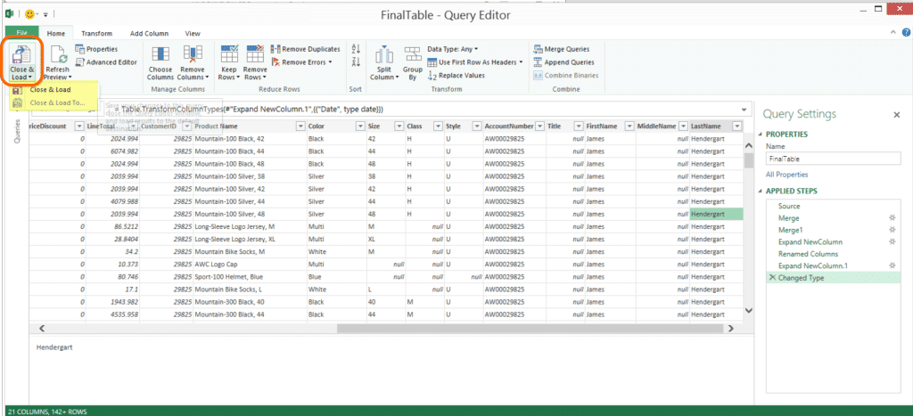
And that’s it! All you have to do now is go to the Home tab, click Close & Load and choose where to land your output (an Excel Worksheet or the Data Model.)
Check the Results Worksheet in the sample file to see the output of the query as constructed in this pattern.