Combine or Append Data from Files

Author: Skillwave Training

The Scenario

If you ever need to:

• Append Data,
• Consolidate Data, or
• Combine Data

that comes from either an Excel, text, or CSV file, then this is the best solution for you to do so.

In this pattern you’ll get the most optimal and easiest way to combine your files from an specific folder and combine them all together if you’d like. That’s right! Combine data from text, CSV, and Excel files all together. There are no limits on the size of the file or how many files you’d like to combine – it’ll simply work!

Our Goal

What we need is a way to extract all the data from our files like:

• CSV Files
• Text Files
• Excel Files

and then somehow consolidate or append data in one tall table. This was a rather complex scenario that we could solve with VBA or SQL, but now we have a more efficient and user friendly way of doing this. Don’t forget to download the workbook in order to follow along!

Step 1: Explaining the Files

Let’s say you have a list of files as shown in the image above, inside a folder called PQExample which is basically the folder where we’re going to point our Power Query solution to work on. The file that contains the actual Power Query solution is called Ultimate Combination.xlsx.

Overall, the files all share the same column header names:

• Product
• Date
• Gross Sales
• Amount

Now we can head over to the real Pattern.

Step 2: Find the Query that does the Magic

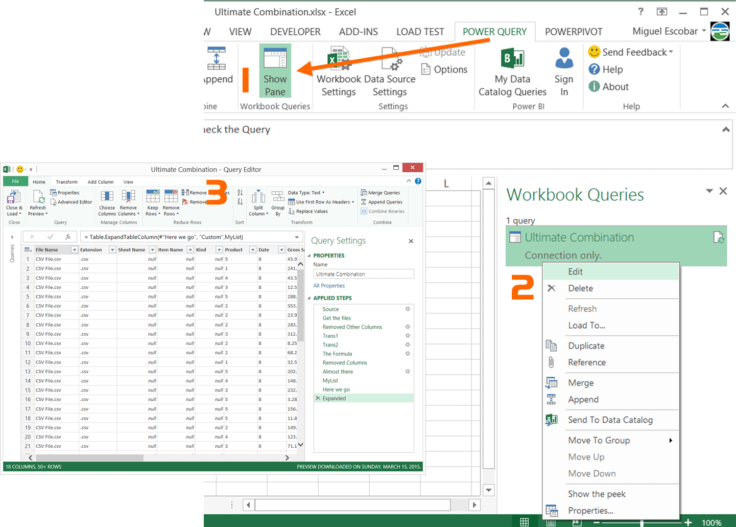
Once you open the Ultimate Combination.xlsx file, you’ll notice that it has no data. The Power Query solution has been stored as a connection only and its awaiting your command to load its data to your Excel workbook. In order to view this query, you’ll need to go to the Power Query ribbon, click on the Show Pane icon and then on the right side you’ll see the Query Pane with a query called Ultimate Combination. Right click that query and then click on Edit to open the Query Editor Window and analyze the solution.

You’ll immediately notice that there is an error with the query, but don’t be alarmed. The reason behind such error its because the solution is pointing at my (Miguel) local folder instead of yours. In order to fix that you’ll need to head over to the first step called Source and click on the gear icon right next to it. That should pop up a new window with a user friendly folder browser. Go ahead and find the folder called PQExample.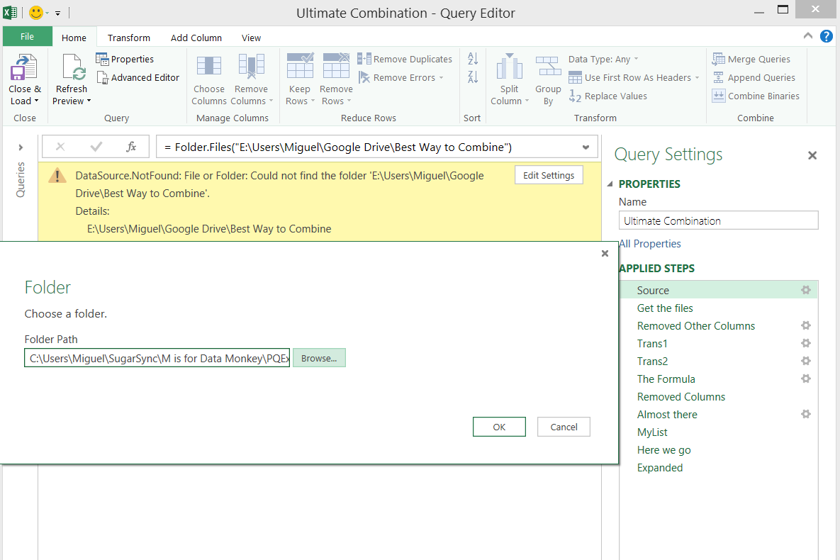
And once you do that, you’ll notice that the solution will start to run and do its magic.

You could end it here and call it a day since all the files were combined already (click on the step called Expanded to see the final result), but instead, we’re going to show how simple creating a solution like this was.

Understanding the Query

Instead of writing a long paragraph, we’ve divided this into sections so you can understand each step of the query on its own.

Source

The way that we start the query is by selecting the folder where all my files are stored. This is easily done through the Power Query Ribbon as shown in the next picture: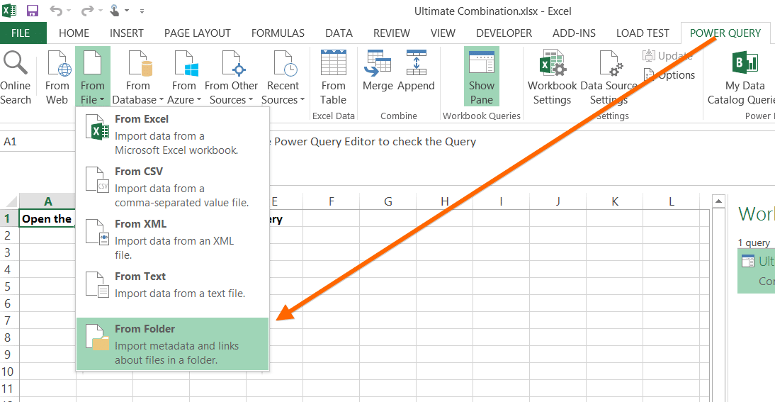
One thing to take in consideration is that Power Query will also grab the files from any subfolder, but you can filter those out by using the Path field.

Get the files

In this step we simply filter the file extension file so we only get the following extensions:

• extension equals .csv
• extension equals .txt
• extension begins with .xls

The way that you’d do this is by selecting the filter icon from the field and simply do a filter like you’d normally do in Excel.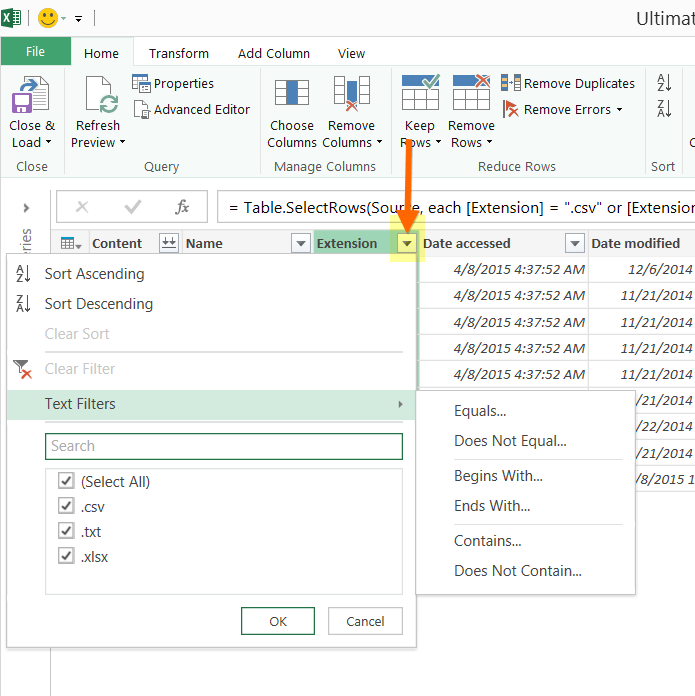

Remove Other Columns

In this case, we’ll be removing some columns that we don’t need. However, instead of selecting the columns that we don’t want, we’ll be selecting the ones that we want and tell Power Query that we just want to keep those. Take a look at the following picture to find the button that does the trick but make sure that you first select the columns that you want to keep.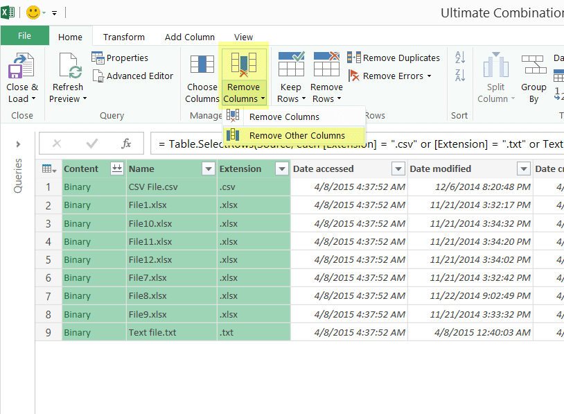

Trans1

Here’s where we’ll need to get to know a bit about Power Query functions. We know that we have some Excel files in our query but, how do we extract the data from them?

Take a look at the columns that we have available. You’ll notice that we have a column called Content that holds a binary. That binary is the actual Excel file and in order to interpret that binary we need a function called Excel.Workbook(). 

Using the following formula:
if Text.StartsWith([Extension], ".xls") then Excel.Workbook( [Content]) else null

we get a new column that is basically the one that shows me all the data that the Excel file (on each row) holds.
You can click on any of the Table values found on the Custom column to find out what’s inside of each of them.
More often, we deal with 3 different kinds of Data inside an Excel Workbook:

1. A Sheet
2. A Table
3. A Named Range

Note: You’ll notice that in some files we’ll have tables, sheets and in others we’ll only have sheets. This is the moment where we define if we just want to combine the tables, the sheets, the named ranges or a combination of them. Be sure to check that you’re not combining the same data twice as a table is part of a sheet and could potentially get combined in the wrong way.

Trans2

Now we need to expand that Custom column so we can get all the Excel data in our Query and choose the ones that we want.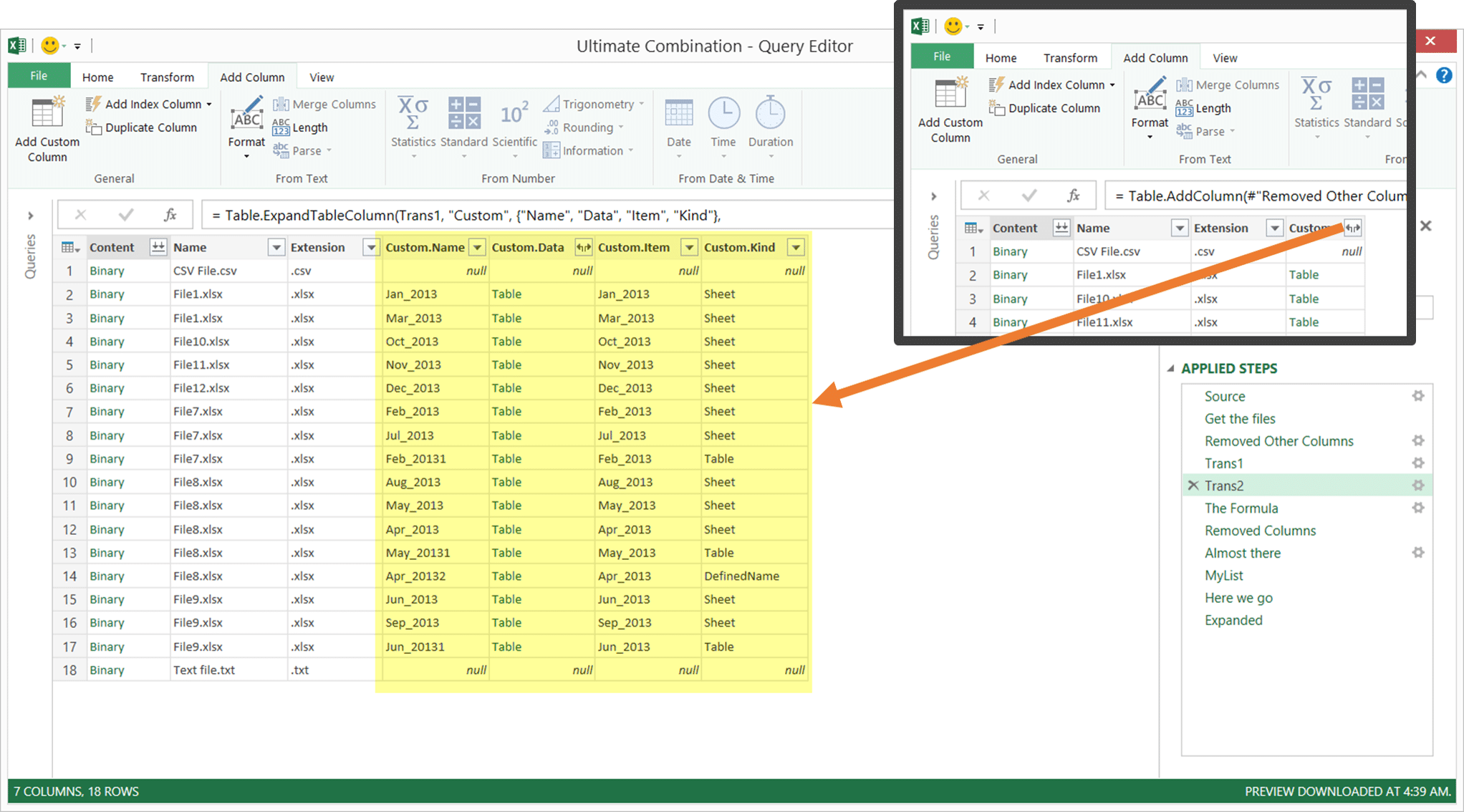
The result of that gives us 4 new columns:

• Custom.Data = the actual data found inside the Excel workbook (represented as a table)
• Custom.Name = the name of the worksheet where the data is stored
• Custom.Item = this is the name of the item, if it’s a named Range then it’ll be the name of that range, for Sheets then it’ll be the name of the Sheet and for Tables it’ll be the name of the table
• Custom.Kind = it’s the name of the object that was found from the excel workbook. Most commons are Sheet, Table and DefinedName

The Formula and Other Steps

So far we managed to extract the data from the Excel workbook into objects. Now we need to find a way to extract the data from the CSV and TXT file and being able to combine that with the data found in the Excel file.

We’ll create a new column with this formula that will do the trick:

if [Extension] = ".csv" then
Table.PromoteHeaders(Csv.Document([Content]))
else if [Extension] = ".txt"
then Table.PromoteHeaders(Csv.Document([Content],null,"," ))
else if [Custom.Kind] <> "Table"
then Table.PromoteHeaders([Custom.Data])
else
[Custom.Data]

Note: we are assuming that the txt file is delimited by a comma, but you can change that by changing the comma in this line of code for something else like a pipe (|), bars (/), semicolon or other.
Csv.Document([Content],null,"," ))

The result of that formula gives us a column that holds only tables with the correct headers. You might be tempted to expand this column right now, but we won’t do that just yet. Instead, we’ll clean the table that we currently have and delete unnecessary columns like Content and Custom.Data since all the data that I need is stored on the Custom column. We will also add a new column that will give us some important information, total row count, about the tables that we’re about to combine. Using this formula we get the total row count for those tables:
Table.RowCount([Custom])

And this is what you see at the Almost there step.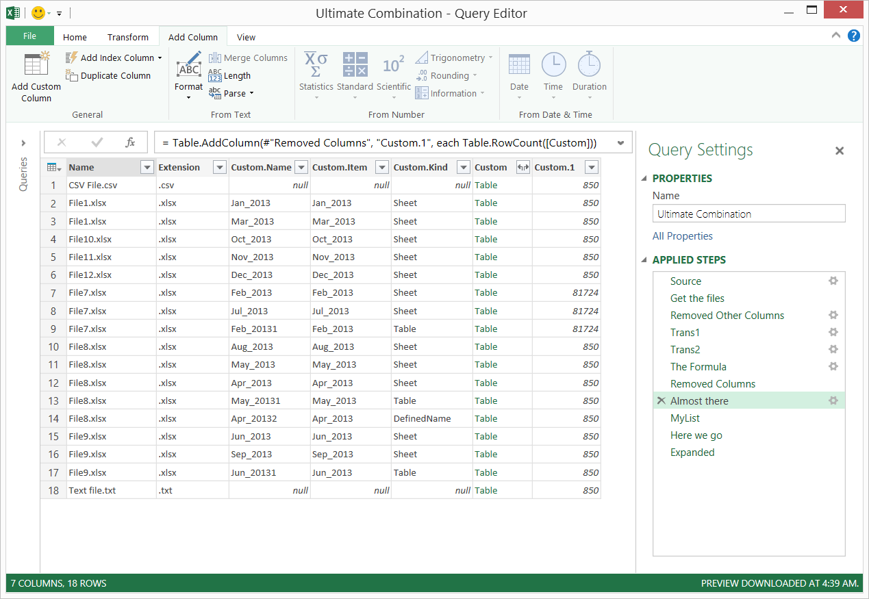

Dynamically Get a List of All Headers in Files

Fundamentally, that’s what the formula at the MyList step does. It basically grabs all the headers from all the tables found in the previous step, gathers them in a table and then creates a table of distinct values. It later transform that Table into a List as we’ll need that List later. That list will become a parameter so we can dynamically combine all the files regardless if they have all the same structure or not.

A common use case to do something like this is that perhaps we have some columns in some files but that are not present in others, but those columns might be needed for that specific analysis and this MyList pattern does just that. It dynamically creates a unique list of all the headers found thorough all the tables in the previous step.

Here’s the code:

=List.Distinct( 
    List.Combine( 
       List.Transform(#"Almost there"[Custom], 
       Table.ColumnNames)
                ) 
  ) 

In order to insert this code you’ll need to create a custom step. You can create a custom step by clicking on the fx icon in the formula bar. Once you activate that custom step, you’ll have to paste the code above to make it work.

This is a custom code that:

1. Converts the column of the previous table that has the “Table” values into a list with just table values
2. What List.Transform does it that it transforms that list into a List of Lists where each list inside that List contains the column names of a specific table
3. List.Combine does just that – it combines all of the lists into a single single
4. List.Distinct is a function that simply remove the duplicated values from a list in order to keep unique values.

This is BY FAR the most efficient way to extract all of the column names from a list of tables. We need this specific list of column names for the final steps.

The Final Steps

The 2 final steps:

• Here we go
• Expanded

The Here we go step simply does some renaming on the columns by just double clicking the name of those columns and the Expanded just simply expands the Custom column by simply clicking on the opposite arrows icon next to the name of that column.

The result of this solution / query should look like this: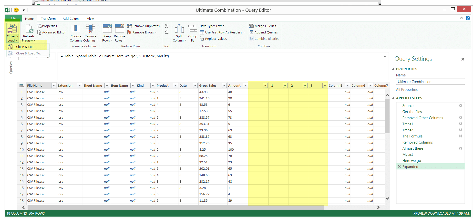


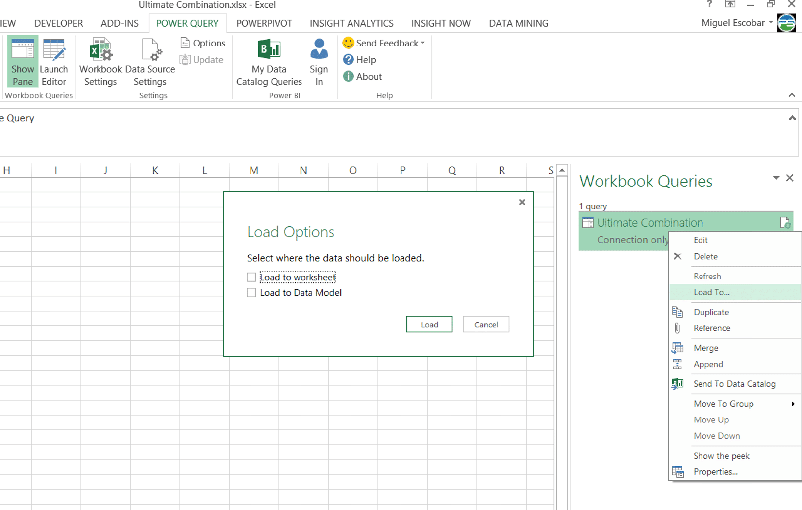
All you have to do now is select where you want to load this, either to a Worksheet or your Data Model!